Motivation
Machine learning models for earth observation often fail in production when they encounter new tiles, different sensors, seasonal changes, or unfamiliar land-cover patterns. seapig helps you manage this uncertainty by enabling selective inference: you can flag uncertain predictions for human review, skip them, or route them to more expensive downstream workflows.
The seapig library provides modular building blocks to score, calibrate, and integrate selective inference into geospatial pipelines—reusing the same logic across segmentation, classification, and regression tasks.
Tutorial overview
This quickstart demonstrates the core five-step workflow using small, interpretable examples:
- Prepare train/val/test splits
- Train a model
- Fit a selection score
- Set a threshold
- Apply selective inference
We use Landsat-8 satellite imagery and Cropland Data Layer labels as the basis of this tutorial. The example is simplified for readability. Production workflows typically require more advanced strategies, such as class balancing, training-time augmentation, and hyperparameter tuning. However, the same pattern works across many task configurations: simply swap the model backend and the selective-inference steps remain unchanged.
Setup
We begin by importing all required libraries and setting random seeds for reproducibility:
import os
import tempfile
from typing import Tuple, List

import torch
from torch.utils.data import DataLoader
from torchmetrics import MetricCollection
from torchmetrics import Accuracy
from lightning import Trainer

from torchgeo.datasets import CDL, Landsat8, stack_samples
from torchgeo.datasets.utils import download_and_extract_archive
from torchgeo.trainers import SemanticSegmentationTask
from torchgeo.samplers import GridGeoSampler, RandomGeoSampler

from shapely.geometry import box, Polygon
import matplotlib.pyplot as plt
import geopandas as gpd

from seapig import SelectiveInferenceTask
from seapig.scores import CosineScore
from seapig.utils import set_backend

set_backend("rich") # progress bars and logging with rich
torch.manual_seed(20260428) # seed for reproducibility
<torch._C.Generator at 0x7f387429d090>
Step 1: Prepare the data
The first step is to gather the input data. We start by downloading Landsat-8 satellite imagery (the model input) and Cropland Data Layer labels (the ground truth), both hosted on HuggingFace. We then combine these into a single dataset that pairs images with their corresponding labels:
url = "https://hf.co/datasets/torchgeo/tutorials/resolve/ff30b729e3cbf906148d69a4441cc68023898924/"
landsat_root = os.path.join(tempfile.gettempdir(), "landsat")
cdl_root = os.path.join(tempfile.gettempdir(), "cdl")

# Download predictors
landsat8_url = url + "LC08_L2SP_023032_20230831_20230911_02_T1.tar.gz"
download_and_extract_archive(landsat8_url, landsat_root)
landsat8 = Landsat8(paths=landsat_root)

# Download targets
cdl_url = url + "2023_30m_cdls.zip"
download_and_extract_archive(cdl_url, cdl_root)
cdl = CDL(paths=cdl_root)

# Combine into (predictor, target) pairs
dataset = landsat8 & cdl
Converting CDL CRS from PROJCS["NAD83 / Conus Albers",GEOGCS["NAD83",DATUM["North_American_Datum_1983",SPHEROID["GRS 1980",6378137,298.257222101,AUTHORITY["EPSG","7019"]],AUTHORITY["EPSG","6269"]],PRIMEM["Greenwich",0,AUTHORITY["EPSG","8901"]],UNIT["degree",0.0174532925199433,AUTHORITY["EPSG","9122"]],AUTHORITY["EPSG","4269"]],PROJECTION["Albers_Conic_Equal_Area"],PARAMETER["latitude_of_center",23],PARAMETER["longitude_of_center",-96],PARAMETER["standard_parallel_1",29.5],PARAMETER["standard_parallel_2",45.5],PARAMETER["false_easting",0],PARAMETER["false_northing",0],UNIT["metre",1,AUTHORITY["EPSG","9001"]],AXIS["Easting",EAST],AXIS["Northing",NORTH],AUTHORITY["EPSG","5070"]] to PROJCS["WGS 84 / UTM zone 16N",GEOGCS["WGS 84",DATUM["WGS_1984",SPHEROID["WGS 84",6378137,298.257223563,AUTHORITY["EPSG","7030"]],AUTHORITY["EPSG","6326"]],PRIMEM["Greenwich",0,AUTHORITY["EPSG","8901"]],UNIT["degree",0.0174532925199433,AUTHORITY["EPSG","9122"]],AUTHORITY["EPSG","4326"]],PROJECTION["Transverse_Mercator"],PARAMETER["latitude_of_origin",0],PARAMETER["central_meridian",-87],PARAMETER["scale_factor",0.9996],PARAMETER["false_easting",500000],PARAMETER["false_northing",0],UNIT["metre",1,AUTHORITY["EPSG","9001"]],AXIS["Easting",EAST],AXIS["Northing",NORTH],AUTHORITY["EPSG","32616"]]
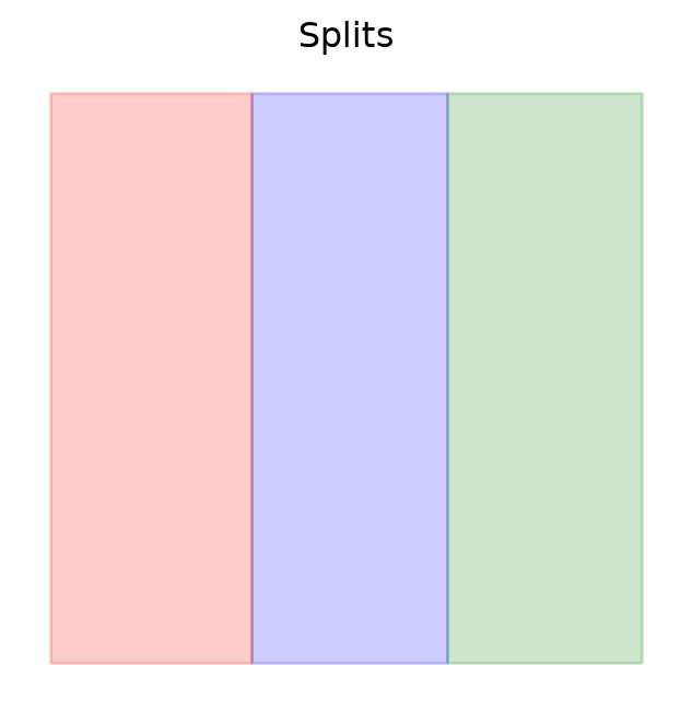
Next, we create geographically distinct train/validation/test splits by dividing the dataset along the x-axis. This is essential for realistic evaluation: we evaluate if a model trained on one part of the landscape generalizes to a different geographic area. We define a function that takes the dataset bounds and splits them into rectangular polygons based on specified size proportions. We also add a margin to avoid sampling near the edges, which can cause issues with patch-based sampling.
Code
def make_split_polygons(
    bounds: tuple,
    size_props: List[float],
    margin: float = 80.0,
    res: float = 30.0
    ) -> Tuple[Polygon, ...]:
    """Split the dataset bounds into train/val/test polygons.

    Produce rectangular Shapely polygons splitting the x-axis of `bounds`
    according to `size_props`. `bounds` is (x_slice, y_slice, t_slice).
    """
    x_slice, y_slice, _ = bounds
    xmin, xmax = float(x_slice.start), float(x_slice.stop)
    ymin, ymax = float(y_slice.start), float(y_slice.stop)

    # we omit one chip on the edges to avoid issues with sampling near the boundaries
    xmin += margin * res
    xmax -= margin * res
    ymin += margin * res
    ymax -= margin * res

    if len(size_props) < 1:
        raise ValueError("size_props must have at least one proportion")
    if abs(sum(size_props) - 1.0) > 1e-6:
        raise ValueError("size_props must sum to 1.0")

    width = xmax - xmin
    cum = 0.0
    polys: List[Polygon] = []
    for p in size_props:
        x0 = xmin + cum * width
        cum += p
        x1 = xmin + cum * width
        polys.append(box(x0, ymin, x1, ymax))

    return tuple(polys)
We apply this function to the dataset bounds, specifying that we want 33% of the data for validation, 33% for testing, and 34% for training:
org_bounds = dataset.bounds
size_props = [0.34, 0.33, 0.33]  # 34% train, 33% val, 33% test
train_poly, val_poly, test_poly = make_split_polygons(org_bounds, size_props)
Let’s visualize the dataset and the spatial splits to ensure they make sense:
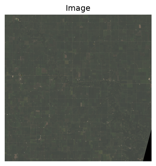
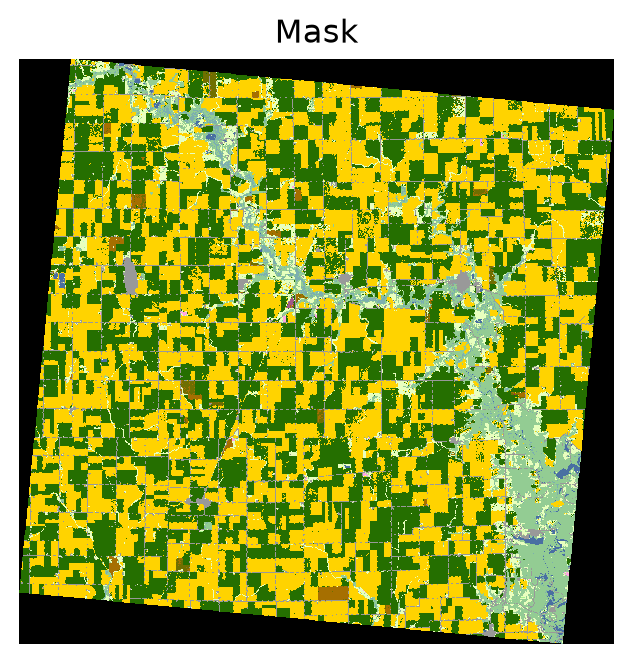
sample = dataset[:]
_ = landsat8.plot(sample)
_ = cdl.plot(sample)
fig, ax = plt.subplots(1, 1, figsize=(4, 4))
gpd.GeoSeries(train_poly).plot(ax=ax, edgecolor="red", facecolor="red", label="train", alpha=0.2)
gpd.GeoSeries(val_poly).plot(ax=ax, edgecolor="blue", facecolor="blue", label="val", alpha=0.2)
gpd.GeoSeries(test_poly).plot(ax=ax, edgecolor="green", facecolor="green", label="test", alpha=0.2)
_ = ax.axis("off")
_ = ax.set_title("Splits")
Step 2: Create data loaders
Now that we have our splits defined, we need to convert them into mini-batches for training. We’ll define samplers for each split using torchgeo, which handles the spatial and temporal complexities of geospatial data:
- Training uses
RandomGeoSampler to randomly sample patches with possible overlaps. This adds variety to the training process and helps the model learn diverse patterns.
- Validation and test use
GridGeoSampler to create non-overlapping grids covering the entire region. This ensures systematic coverage without gaps, which is important for consistent evaluation.
We use 16×16 pixel patches, a small size chosen for demonstration (the full scene is ~1024×1024 pixels):
train_sampler = RandomGeoSampler(dataset, roi=train_poly, size=16)
val_sampler = GridGeoSampler(dataset, roi=val_poly, size=16)
test_sampler = GridGeoSampler(dataset, roi=test_poly, size=16)

print(f"Train samples: {len(train_sampler)}")
print(f"Val samples: {len(val_sampler)}")
print(f"Test samples: {len(test_sampler)}")
Train samples: 988
Val samples: 936
Test samples: 936
Next, we wrap these samplers in PyTorch DataLoaders with stack_samples as the collate function. The collate function handles the correct stacking of geospatial samples to form mini-batches:
train_dl = DataLoader(dataset, batch_size=4, sampler=train_sampler, collate_fn=stack_samples)
val_dl = DataLoader(dataset, batch_size=4, sampler=val_sampler, collate_fn=stack_samples)
test_dl = DataLoader(dataset, batch_size=4, sampler=test_sampler, collate_fn=stack_samples)
Step 3: Train a model
To train a model, we define a MySegmentationTask class that inherits from torchgeo’s SegmentationTask. This class specifies how to perform a forward pass, compute the loss, and calculate metrics. We extend this class by implementing the embed method, which generates embeddings from the model’s encoder. These embeddings are crucial for fitting the selection score later on. Additionally, we override the configure_metrics method to set up appropriate metrics for evaluating the segmentation performance:
Code
class MySegmentationTask(SemanticSegmentationTask):
    """A simple segmentation task with an embedding method for selective inference."""
    def __init__(self, *args, **kwargs):
        super().__init__(*args, **kwargs)

    def embed(self, x: torch.Tensor) -> torch.Tensor:
        """Generate embeddings from the model's encoder for use in selection scoring."""
        x = x.to(next(self.model.parameters()).device)
        embs = self.model.encoder(x)[-1]
        embs = torch.mean(embs, dim=(-2, -1)) + torch.amax(embs, dim=(-2, -1))
        embs = torch.nn.functional.normalize(embs, p=2, dim=1, out=embs)
        return embs

    def configure_metrics(self) -> None:
        """Configure metrics for training, validation, and testing."""
        kwargs = {
            "task": self.hparams["task"],
            "num_classes": self.hparams["num_classes"],
        }
        metrics = MetricCollection(
            {
                "Accuracy": Accuracy(average="micro", **kwargs),
            }
        )
        self.train_metrics = metrics.clone(prefix="train_")
        self.val_metrics = metrics.clone(prefix="val_")
        self.test_metrics = metrics.clone(prefix="test_")
Now we train a segmentation model that learns to classify each pixel as a crop type. We use a minimal UNet architecture with a ResNet18 backbone. This configuration is intentionally simple for tutorial clarity; in production, you’d possibly add data augmentation, longer training schedules, and careful hyperparameter tuning:
model = MySegmentationTask(
    model="unet",
    backbone="resnet18",
    weights=True,
    in_channels=len(landsat8.bands),
    task="multiclass",
    num_classes=len(cdl.classes),
    loss="ce",
    lr=1e-3,
)
trainer = Trainer(max_epochs=1, accelerator="cpu")
trainer.fit(model, train_dl, val_dl)
┏━━━┳━━━━━━━━━━━━━━━┳━━━━━━━━━━━━━━━━━━┳━━━━━━━━┳━━━━━━━┳━━━━━━━┓
┃   ┃ Name          ┃ Type             ┃ Params ┃ Mode  ┃ FLOPs ┃
┡━━━╇━━━━━━━━━━━━━━━╇━━━━━━━━━━━━━━━━━━╇━━━━━━━━╇━━━━━━━╇━━━━━━━┩
│ 0 │ model         │ Unet             │ 14.4 M │ train │     0 │
│ 1 │ criterion     │ CrossEntropyLoss │      0 │ train │     0 │
│ 2 │ train_metrics │ MetricCollection │      0 │ train │     0 │
│ 3 │ val_metrics   │ MetricCollection │      0 │ train │     0 │
│ 4 │ test_metrics  │ MetricCollection │      0 │ train │     0 │
└───┴───────────────┴──────────────────┴────────┴───────┴───────┘
Trainable params: 14.4 M
Non-trainable params: 0
Total params: 14.4 M
Total estimated model params size (MB): 57.440
Modules in train mode: 147
Modules in eval mode: 0
Total FLOPs: 0
/home/runner/work/seapig/seapig/.venv/lib/python3.12/site-packages/lightning/pytorch/utilities/_pytree.py:21:
`isinstance(treespec, LeafSpec)` is deprecated, use `isinstance(treespec, TreeSpec) and treespec.is_leaf()`
instead.
/home/runner/work/seapig/seapig/.venv/lib/python3.12/site-packages/lightning/pytorch/trainer/connectors/data_connec
tor.py:434: The 'val_dataloader' does not have many workers which may be a bottleneck. Consider increasing the
value of the `num_workers` argument` to `num_workers=3` in the `DataLoader` to improve performance.
/home/runner/work/seapig/seapig/.venv/lib/python3.12/site-packages/lightning/pytorch/utilities/_pytree.py:21:
`isinstance(treespec, LeafSpec)` is deprecated, use `isinstance(treespec, TreeSpec) and treespec.is_leaf()`
instead.
/home/runner/work/seapig/seapig/.venv/lib/python3.12/site-packages/lightning/pytorch/trainer/connectors/data_connec
tor.py:434: The 'train_dataloader' does not have many workers which may be a bottleneck. Consider increasing the
value of the `num_workers` argument` to `num_workers=3` in the `DataLoader` to improve performance.
Step 4: Fit and calibrate a score
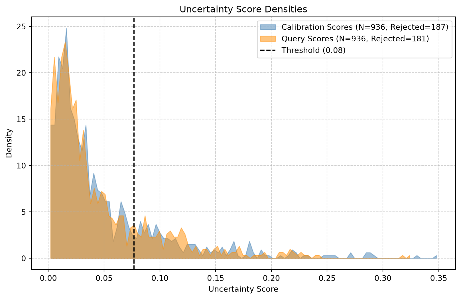
Here’s where seapig comes in. A selection score quantifies how uncertain the model is in each prediction. We use CosineScore, which measures the distance between a query embedding and its nearest neighbor in the training embedding space. Lower scores indicate that a sample is similar to training data (lower uncertainty), while higher scores indicate the model has encountered something unfamiliar (higher uncertainty).
We fit the score on both training and validation data, so it learns what “normal” and “unusual” look like. Then we set a threshold at the 80th percentile of the validation score distribution. This means the model will flag roughly the top 20% most uncertain predictions:
score = CosineScore(k=1)
score.fit(model=model, loaders={"train": train_dl, "val": val_dl})
score.set_threshold(q=0.80)
print(f"Threshold: {score.threshold}")
Threshold: 0.07669562101364136
Step 5: Apply selective inference
Finally, we apply selective inference on the test set. This step separates predictions into two categories based on whether their score falls below or above the threshold:
test_selection = score.select(model=model, loader=test_dl)
score.plot(query_scores=test_selection["score"])
We can wrap the model and score into a unified SelectiveInferenceTask. This container computes performance metrics separately for selected and rejected samples. This breakdown reveals where the model is reliable (selected) and where it struggles (rejected), providing actionable insights for deployment:
sel_model = SelectiveInferenceTask(task=model, score=score, input_key='image', target_key='mask')
stats = trainer.test(sel_model, test_dl)
/home/runner/work/seapig/seapig/.venv/lib/python3.12/site-packages/lightning/pytorch/utilities/_pytree.py:21: `isinstance(treespec, LeafSpec)` is deprecated, use `isinstance(treespec, TreeSpec) and treespec.is_leaf()` instead.
/home/runner/work/seapig/seapig/.venv/lib/python3.12/site-packages/lightning/pytorch/trainer/connectors/data_connector.py:434: The 'test_dataloader' does not have many workers which may be a bottleneck. Consider increasing the value of the `num_workers` argument` to `num_workers=3` in the `DataLoader` to improve performance.
┏━━━━━━━━━━━━━━━━━━━━━━━━━━━┳━━━━━━━━━━━━━━━━━━━━━━━━━━━┓
┃        Test metric        ┃       DataLoader 0        ┃
┡━━━━━━━━━━━━━━━━━━━━━━━━━━━╇━━━━━━━━━━━━━━━━━━━━━━━━━━━┩
│    full/test_Accuracy     │    0.6230218410491943     │
│  rejected/test_Accuracy   │    0.4837707281112671     │
│  selected/test_Accuracy   │    0.6564052104949951     │
└───────────────────────────┴───────────────────────────┘
What is left now is to get predictions and selection results for the entire domain an stitch the batchs together to produce geospatial maps. There are ongoing efforts in torchgeo to support this kind of geospatial post-processing directly within the library (see this issue thread to find some pointers). Until this is available upstream, one has to manually stitch together the outputs from the dataloader. We are going to cover this in an upcoming tutorial.